
Chapter 02: Application of Economic Principles to Market Definition
Application of Economic Principles to Market Definition
“In general, if any branch of trade, or any division of labour, be advantageous to the public, the freer and more general the competition, it will always be the more so.”
Adam Smith, from The Wealth of Nations
This chapter is intended to provide the basic economic principles needed to analyze agricultural markets. Ideally a student will have already mastered the principles discussed in this chapter; however, the author has included this chapter in recognition of the fact that this is seldom the case. In some cases, the student will not have taken an economics course. More often the economics course or courses taken were either poorly taught, lacked real world examples to illustrate the crucial real-world importance of the topic, or the student, failing to recognize the importance of the class, was not paying attention.
Economics involves choices because resources are scarce. Even if we were incredibly wealthy, making choices would still be necessary because everyone has only a limited amount of time. Average life expectancy in the United States is 76.4 years according to government statistics.1 An individual’s life expectancy will be determined by such factors as gender, race, socioeconomic status, and many other factors. Nonetheless the amount of time that all of us have is limited. All of us must decide how to allocate the resources that we have.
1 76.4 is life expectancy at birth for a person born in 2020. A person that is between 76 and 77 years of age in 2020 has a life expectancy of about 87 (10.9 additional years). To understand this please review the life tables published by the CDC (referenced at the end of this chapter).

Figure 2.1 : A market-place
Khan Academy video on scarcity
The science of economics helps us make those choices. It also helps us predict the economic consequences of policy choices. Example 2.1 illustrates how policy choices in states that have legalized cannabis are likely to allocate the market for cannabis between legal operators and illegal operators. Understanding these concepts is of critical importance to policy and legislation and the private businesses that must navigate markets.
With the repeal of prohibition, federal bureaucrats turned their focus to marijuana. What follows is the propaganda film “Reefer Madness” – play time 1 hour and 8 minutes.
Example 2.1. As happened with the end of Prohibition2 and the legalization of alcoholic beverages, legalized cannabis (marijuana) faces a substantial tax burden. The effect of this is to place a price floor under illegal cannabis. This has worked as a price support for illegal cannabis producers. The lessons from the end of Prohibition were not learned. The Eighteenth Amendment, ratified January 16, 1919, prohibited legal production, importation, transportation and sale of alcoholic beverages. Legalization through the Twenty-first Amendment was accompanied by high “sin” taxes on alcoholic beverages. These taxes created a floor under the price of illegal “moonshine” alcohol that has allowed moonshine businesses to operate profitably to this day. The same pattern is holding true for marijuana.
2 From 1920 until 1933, the manufacture, import or export, sale, transportation of intoxicating liquors (alcoholic) was banned in the United States under the terms of the 18th Amendment to the Constitution. The 18th Amendment was implemented through the Volstead Act that became effective in 1920. In March 1933, President Franklin Roosevelt signed the Cullen-Harrison Act that allowed the sale of low (3.2%) alcohol beer. On December 5, 1933, ratification of the 21st Amendment repealed prohibition at the federal level. The 21st Amendment allowed prohibition at the state and local level.

Figure 2.2 :
PERFECT COMPETITION
Figure 2.3 illustrates a competitive equilibrium in a perfectly competitive market. No such markets exist in the real world. A perfectly competitive market is an important economic model. The value of the concept of a model is that it provides a baseline against which existing markets can be measured. Models simplify reality in ways that make it possible to understand complex systems. The model allows market participants to answer such questions as ‘If I increase the price of my product will my revenue increase?’ Getting the answer to that question wrong can be catastrophic for a business. If the answer is that customers will quit buying after a price increase, it may not be possible to save the business by making a price cut. Customers may be reluctant to return after they have found other suppliers. The model of a perfectly competitive market can also be used to advice policy makers about how to structure a legal cannabis market if they wish to minimize the illegal market.
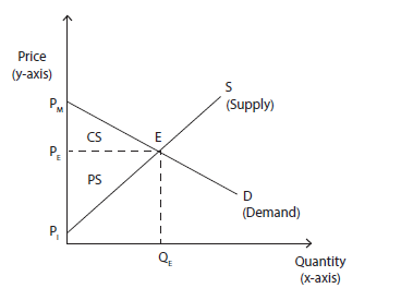
Figure 2.3 : Perfectly competitive widget market
In a perfectly competitive market, there are a sufficient number of buyers and sellers that no market participant has the market power to set prices. The good sold is homogenous. Example 2.2 illustrates a homogeneous good. There must be freedom of entry and exit from the market and information must be perfect, i.e., no participant has better information than any other participant.
Example 2.3 provides a real-world example of the value of imperfect information to those with information superior to other market participants. An additional condition is that there are no market distorting conditions. Examples of conditions that distort markets include needs of national defense, taxation, regulation to protect the environment and worker safety, incentives to encourage innovation such as patents, federal farm programs, and programs subsidizing food purchases by the poor. Market distortions are neither good nor bad per se. Market efficiency is only one of several facts to evaluate in making policy decisions.
As Figure 2.3 shows, a perfectly competitive market for a widget3 is defined by an upward sloping supply curve and a downward sloping demand curve. For our widget, its price is on the y axis, and quantity demanded is on the x axis. The supply curve (S) slopes upward because producers are willing to supply more of a good at a higher price. The demand curve, D, slopes downward because consumers will buy more as the price drops. PE, where the demand and supply curves intersect, is the market clearing (equilibrium) price. It is the price that all sellers receive, and all buyers pay, in a perfectly competitive market. QE is the quantity of widgets provided at price PE.
3 A fictional good for a theoretical perfectly competitive market that does not exist.

Figure 2.4 :
Khan Academy video on market equilibrium.
The demand and supply curves pictured in Figure 2.3 are aggregate demand and supply curves. Looking at the supply curve, there is at least one seller willing to sell at P1. Note that this price is above zero. That the supply curve begins above zero reflects that below P1, there is no seller willing to sell a widget. Along the section of the supply curve defined by P1 to PE, there are sellers willing to sell at a price below PE. Since all goods in a perfectly competitive market are sold at the equilibrium price, PE, all sellers willing to sell at a lower price receive a windfall, that we call the producer surplus. For our aggregate demand and supply curves illustrated in Figure 2.3, the aggregate producer surplus, labeled PS, is defined as the triangle bounded by P1 to PE on the y axis, P1 to where the demand and supply curves cross (E, the equilibrium between demand and supply), and the dashed line from PE to point E. The area within this triangle is labeled PS, the producer surplus.

Complete this khan Academy exercise.
In a similar manner, the consumer surplus, in the area labeled CS, is defined by the triangle bounded by PM to PE on the y axis, the section of the demand curve defined by PM to E, and the dashed line from PE to point E. The distance between PE and PM (the maximum price that any consumer would pay) is the windfall that any consumer willing to price PM would receive. The aggregate consumer surplus is the sum of all amounts above PE that consumers would be willing to pay for a widget. For consumers and sellers willing to trade only at PE, there is no surplus.
The sum of PS and CS gives us total surplus, TS. Maximizing TS gives us an efficient market that provides the most goods to the most consumers at the lowest possible cost. The value of this model is it gives us a vehicle for measuring the loss of efficiency associated with less efficient market structures. Efficiency is one way of measuring market performance. There are others that include resilience, national security, raising tax revenue, and equity. These other measures are much more difficult to define than efficiency and therefore much more difficult to measure.
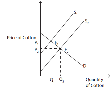
Figure 2.5 : Impact of invention of the cotton gin on the cotton woven for cotton
What we can measure is the loss of efficiency associated with these other market structures. The value of measures other than efficiency are often the source of a great deal of political conflict. As Adam Smith stated 300 years ago, the purpose of production is to benefit consumers. Anything that reduces consumer welfare should be viewed with skepticism unless compelling reasons can be shown for the policy.

Figure 2.6 :
4 The cotton gin mechanically separates the cotton fiber from the seeds. Prior to its invention this step was done by hand.
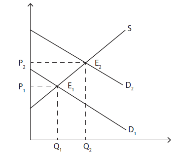
Figure 2.7 : Impact of printed cotton t-shirt on the demand for cotton
Figure 2.7 illustrates an upward shift in demand caused by the introduction of printed cotton T-shirts. The introduction of printed cotton T-shirts increased the demand for cotton that is reflected in the movement of the demand curve upward from D1 to D2. The supply curve, S, did not change. The market equilibrium shifted upward and outward from E1 to E2. Price increased from P1 to P2, and quantity increased from Q1 to Q2.
Example 2.2. For our model to work it must refer to a good that is sufficiently well-defined that it excludes all similar goods. To illustrate how this works let us take as an example, ‘Wheat, Spring 14%-pro Mnpls; $/bu. – U’. ‘Wheat’ means grain produced from the seed of a grass in the genus, Triticum. There are many species of wheat. ‘Spring’ means that it is planted in the spring and harvested in the summer. The other major class of wheat is ‘winter’ wheat that is planted in the fall, grows over the winter, and is harvested in the late spring or early summer. ‘14% pro’ is the minimum protein content. ‘Mnpls’ refers to the price at the Minneapolis, Minnesota, market. ‘U’ is short for USDA which is the source of this particular price series. This is a cash price in contrast to a price for future delivery. Chapter 7 provides details about the market for agricultural commodities. Chapter 9 discusses grades and standards that are critical to defining what product is being bought and sold. Chapters 13, 14, and 15 provide details about the various ways that a farmer may use to sell agricultural commodities. Some of this has been discussed briefly in chapter 8 in the discussion of milk markets.
Example 2.3. Spread Networks completed a fiber optic line in 2010 that connected the futures markets in Chicago with the stock markets of New York. The result was reducing the time required for information to travel between the two markets by 3 milliseconds (three-thousands of a second). The cost of this line was estimated at $300 million. With computerized trading in futures and stock markets, the better information provided to traders (speculators) using the line was well worth the cost. The benefits to private speculators are clear. It is not clear that society as a whole benefits. It is likely that this is an example of how market distortions reduce the welfare of society. Another way of saying this is that $300 million dollars could have provided improvements to many schools which might have been a better use of society’s limited resources.
MARKET POWER AND PRICE ELASTICITY
Now that we have introduced the model of the perfect competition, we will address how economics can help businesses determine whether or not a price increase would be beneficial. This concept is called elasticity. It is defined as how responsive one variable is to a change in another variable.
Price elasticity of demand
Khan Academy video on price elasticity of demand.
Price elasticity of demand measures how consumers respond to a change in the price of widgets. There are three possible responses. First, a one percent increase in price could result in a one percent decrease in units sold, with no change in revenue.5 This is called unitary elasticity because revenue does not change in a response to a change in price. Second, a one percent increase in price could result in a reduction in units sold of less than one percent, with an increase in revenue. This is called inelastic because the percentage drop in units sold is less than the percentage increase in price. Third, a one percent increase in price could result in a reduction in units sold of more than one percent, with a decrease in revenue. This is called elastic because the percentage drop in units sold is more than the percentage increase in price.
5 All revenue in this discussion is gross revenue (revenue before subtracting expenses). Net revenue (profit) will be determined for each firm by each firm’s individual cost structure.
The availability of substitutes determines the price elasticity of particular goods. Substitutes are goods that are close enough in character that they can be used interchangeably without significantly affecting consumer utility. Perfect substitutes are goods that can be used interchangeably without any reduction in consumer utility. Perfect substitutes are rare. In most cases substitutes are imperfect matches for each other.
Example 2.4. Cigarettes are an example of a category of goods that are extremely price inelastic. Cigarettes contain nicotine, an addictive substance. Smokers will go to extremes to obtain cigarettes. Smokers have a great deal of brand loyalty which makes different brand imperfect substitutes. Although the demand for a particular brand is more elastic than the demand for cigarettes as a whole, the elasticity of demand for particular brands is less than might be expected due to brand loyalty.
Example 2.5. Agricultural commodities of a particular grade, such as the wheat described in Example 2.2 are close to being perfectly elastic; however, there are permissible tolerances within grades. There may also be differences in transportation costs. This leaves open that all wheat of the same grade may not be perfect substitutes. A wheat farmer that can sell a large buyer 500 tractor trailer loads of wheat will usually be preferred to 50 farmers that can provide 10 loads each. The buyer’s truckers need become familiar with only a single loading facility as opposed to 50. It is easier to work with one buyer to ensure tighter tolerances than required by a grade. U.S. Number 1 wheat is limited to no more than 0.4% foreign matter. If the buyer needs wheat that is no more than 0.2% foreign matter, it is much easier (and less costly) to achieve while working with one farmer as opposed to 50. What one sees is that large farmers who are willing to sell to a single buyer are able to get a premium to the market price that reflects the buyer’s reduction in costs associated with buying from a high-volume producer.

Figure 2.8 :
Price elasticity of supply
Price elasticity of supply is the flip side of price elasticity of demand. It reflects suppliers’ response to a change in the price of the goods that they sell.
Income elasticity
Income elasticity measures how consumers respond to a change in income. Normal goods experience an increase in demand as consumer income increases. Two subcategories of normal goods are necessities and luxuries. Necessities have a small positive increase in demand as income increases. Food is the classic example of a normal good. A luxury good is one that has increasing demand as income increases. Inferior goods are not normal goods. They show decreasing demand as income decreases.
Example 2.6. Beans are an example of goods that behave as necessities over the lower part of the range of consumer incomes. Beans are inferior goods for higher income consumers. For lower income consumers, beans show slightly increasing demand as income increases. At income levels where consumers can afford preferred sources of protein such as steak, demand for beans declines as income increases. Certain varieties of beans, usually certified organic heirloom varieties, may behave as luxury goods, with demand increasing as income increases. This example illustrates the need for careful analysis of the characteristics of particular goods to determine their demand behavior as income changes.

Figure 2.9 :
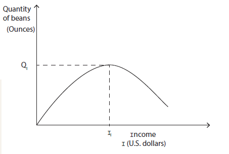
Figure 2.10 : Engel curve
6 Some luxury goods are more costly to produce than other normal goods. Some have higher quality or unique characteristics. However, all have the characteristic of exclusivity.
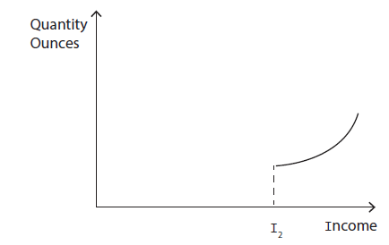
Figure 2.11 : Luxury good (certified organic heirloom beans)
Cross-price elasticity of demand
Cross-price elasticity of demand measures how much a change in demand for one good changes the price of another good. Substitutes have a positive cross price elasticity of demand. When the price of one good goes up the demand for a substitute will go up. Contrast this with complementary goods. Hot dogs and buns are the classic example of complementary goods. If the price of hot dogs goes up, the amount of both hot dogs and buns demanded will fall.
Cross-price elasticity of supply
Cross-price elasticity of supply measures how supply of one good changes in response to a change in price of another good. For substitutes the cross elasticity of supply is negative.
Example 2.7. If farmers have the equipment for raising and harvesting both soybeans and corn, then those crops are substitutes for each other. The choice of which to grow will depend on a number of factors, one of which is price. All other factors being the same, farmers will choose to grow more of the crop with the higher expected price. There are other factors that will affect this decision. These factors include risk management (both price and production risk), disease and weed control through crop rotation, and whether the farm has an associated livestock operation that uses the corn on the farm.

Figure 2.12 :

Figure 2.13 :
Complementary goods have a positive cross elasticity of supply. A drop in the price of hot dogs increases both hot dogs sold, and the number of buns sold. For goods that are neither substitutes nor complementary the cross elasticity of supply is zero.
Example 2.8. Example 2.8. Hot dogs typically come in packs of 10 while buns come in packs of 8 or 12. Since hot dogs and buns are complementary goods one would logically expect the packages to be of the same size. Historically that has not been the case. Economists have given this and other similar anomalies serious study! As with much of what economists do, they came to no definitive conclusion. Readers will be happy to know that the food company, Heinz, has proposed the 2013 Heinz Hot Dog Pact to persuade producers to standardize packaging of hot dogs and buns on 10 items per package.

Heinz Hot Dog pact.
How To Understand Elasticity
UNDERSTANDING MARKET POWER
Market power is the ability of a seller to determine the price that it receives. It is also possible for buyers to have market power (called a monopsony) that allows them to determine the price they pay for goods. This section will discuss both along with different sources of market power. It is always in the interest of businesses to have market power because it increases net revenue. Market power generally reduces the efficiency of markets.
Market power is also called monopoly power. As a technical matter, a monopoly is a single firm that produces a good or provides a service for which there are no close substitutes. It is rare for a single firm to produce a good for which there are no close substitutes. More often there are a few producers making similar goods or providing similar services. These firms have some market power and engage in what is known as monopolistic competition. The extent of each company’s market power will depend on the structure of the industry, which will be discussed later in this chapter. For now, we will focus on a single company that is a monopoly. If the monopolist sets the price of the good, the demand curve will determine the quantity that buyers purchase. In the alternative the monopolist sets the quantity the demand curve will determine the price. A monopolist can set price or quantity but not both.
A monopolist maximizes profits by producing at the level where the difference between total revenue (TR) and total cost (TC) is greatest. The profit maximizing point may also be described as the point where marginal revenue equals marginal cost. Marginal revenue is defined as the additional revenue from each additional unit of product produced. Marginal cost is the additional cost of each additional unit of product. A rational producer will continue to produce more units so long as the difference between marginal revenue and marginal cost is positive.
Figure 2.14 illustrates a profit maximizing monopolist. Total revenue (R1) is maximized at the peak of the total revenue curve; however, that is not the profit maximizing point. The difference between total revenue and total cost is maximized at a lower level of production, Q2. The shape of the total revenue curve is determined by elasticity of demand. Elasticity of demand is unitary at the peak of the total revenue curve (R1). The section of the demand curve that corresponds to the quantities of up to Q1 on the total revenue curve is inelastic. When the demand curve is inelastic, an increase in price produces an increase in total revenue. Beyond Q1 the demand curve is elastic. Over this part of the demand curve the relationship between price and total revenue is negative. A demand curve with these characteristics produces the downward sloping parabola of Figure 2.14.
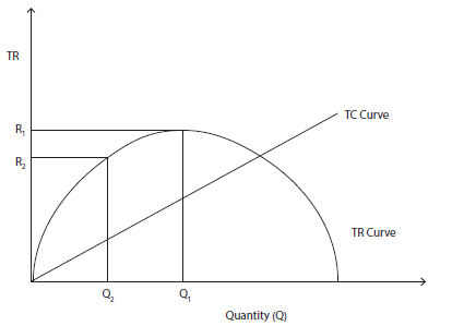
Figure 2.14 : Maximizing monopoly profits
Contrast a firm in a perfectly competitive market with a monopolist. If a firm in a perfectly competitive market raises its price, it will sell nothing. A monopolist has pricing power. How much depends upon the elasticity of demand discussed in the previous paragraph. Monopolists selling products that are price elastic will not be able to charge high markups. Where the elasticity of demand is inelastic, the seller can choose much higher markups.
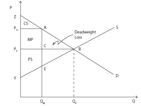
Figure 2.15 : Deadweight loss
Figure 2.15 illustrates efficiency losses as the result of monopoly power. In a perfectly competitive market, quantity QP would be produced at PP. The monopolist produces QM at PM. The result is to transfer consumer surplus, labeled MP, to the monopolist as monopoly profits. Consumer surplus, a triangle bounded by points A, B, and C, and producer surplus, bounded by points B, C, and E, no longer exists. Called deadweight loss, this is the efficiency cost of monopoly.
Unlike a firm in a perfectly competitive market, a monopolist faces no supply curve because there is not a one-to-one correspondence between price and quantity supplied. Prices for monopolists depend upon the shape of the demand curve.
Monopolies may be either discouraged or encouraged by government policy. Farmers are encouraged to form monopolies through cooperatives to counteract monopoly power of buyers and suppliers. Inventors are given patent protection to encourage innovation. Monopolies based upon anticompetitive practices, such as price fixing, are usually against the law.
Example 2.9. Lysine is an essential amino acid traded on world markets. Five companies, dominant in the market, agreed to set a uniform price higher than the market price. The companies were successfully prosecuted, and four executives were prosecuted, convicted under the 1890 Sherman Act, and sent to prison.

Figure 2.16 :
What is a Monopoly?
STRATEGIES USED BY FIRMS WITH MARKET POWER
Khan Academy on types of competition
Price discrimination
First degree price discrimination
A perfect monopolist would charge each buyer the maximum amount that each was willing to pay. This is first degree price discrimination, the most extreme form of price discrimination. The maximum amount that each buyer will pay is called the reservation price. Charging all buyers their individual reservation prices would capture the entire consumer surplus under the demand curve that corresponds to the area where the marginal revenue exceeds the marginal cost.
Example 2.10. Arnold smuggled a package of 10 candies into summer camp where candy was not available. He purchased the box of candies for $10 dollars. In this example, marginal cost and average cost are equal and equal to one dollar. He auctioned the candies off to his fellow campers, starting with the highest bid. He sold one to Joe for $5, one to Mary for $4, one to Jeff for $3, one to Susan for $2, and one to Peter for $1. Poor Paul had only 75 cents to bid. Arnold rejected his bid as below what he had paid for the candies. He decided to eat the remaining five candies himself. Arnold sold candies to each of his fellow campers until marginal cost equaled marginal revenue. Below that point he refused to sell. Arnold engaged in what economists call perfect price discrimination.
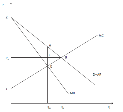
Figure 2.17 : Perfect price discrimination
Figure 2.17 illustrates perfect price discrimination. Note the important difference between Figure 2.17 and Figure 2.15. In Figure 2.17, there is no single monopoly price. By charging each buyer the maximum that each is willing to pay, the monopolist has captured the entire consumer surplus. The deadweight loss bounded by A, B, and E remains the same as in Figure 2.15. This loss is reflected in the fact that the monopolist will not sell at the prices on the demand curve represented the section of the demand curve between points A and B because for those prices, the monopolist’s marginal revenue (MR) is less than its marginal cost (MC).
There are practical and legal obstacles that prevent monopolists from achieving the objective of perfect price discrimination. It is often expensive or impossible to determine the maximum price that each buyer is willing to pay. Various laws governing commerce (e.g., antitrust and unfair business practice laws) typically make it illegal to charge each buyer a different price. Most monopolists that engage in price discrimination engage in what is called imperfect price discrimination. Companies engaging in imperfect price discrimination are able to identify different groups of customers with different willingness to pay.7 These different groups can be charged different prices.
7 In the case of advertising, discussed below, they may create such groups.
Second degree price discrimination
A quantity discount is a more common name for second degree price discrimination. Larger quantities of a product are typically sold for a lower per unit price. Buyers with limited storage space or limited consumption will generally be willing to pay a higher per unit price than a buyer with more storage space or a family that will consume at a faster rate than a single person.
Third degree price discrimination
Third degree price discrimination different groups of consumers different prices based upon the willingness of each group to pay. Student discounts, senior discounts, and other discounts for identifiable groups are all examples of thirddegree price discrimination.
Example 2.11. To the annoyance of their customers, airlines are well known for engaging in price discrimination. They separate business and leisure travelers because leisure travelers are more price sensitive than business travelers. Business travelers pay considerably more for the same travel (although they may receive certain perks such as better seating and free alcoholic beverages.) The COVID-19 pandemic may have permanently disrupted that business model by shifting a significant portion of business meetings to an online format. It remains to be determined whether the shift is permanent.

Time of day price discrimination

Figure 2.18 :
Intertemporal price discrimination
Intertemporal price discrimination uses time as the factor that distinguishes groups of buyers. Sellers of technology products and services often use this form of price discrimination. When a product is initially introduced, the price will be higher than the price at which it is sold some months later. Certain new models of cell phone are a good example of technology products marketed in this way.
Peak load pricing
For some products and services, there are predictable times when those products or services are more in demand. Roads and electricity are both subject to peak loads.
Example 2.12. Peak electricity demand over the course of a day varies by region and between summer and winter. Summer peak hours in the Eastern time zone are 2 PM to 6 PM and for winter, 6 AM to 10 AM, and 6 PM to 10 PM. Richard operates a feed mill. He agreed to a lockout for his mill during peak hours. This allows for substantial savings in electric use charges.
Two-part pricing
Under two-part pricing the consumer is charged both a fixed price and a per-unit price. This is usually in the form of an entry fee and a charge for service or product once the entry is made.
Example 2.13. Richard uses the feed that he makes in his mill to feed fish on his fish farm. He raises rainbow trout. His ponds are open to the public for fishing at a price of $10 per day or $100 per person for the season with a family discount of 50%. Children under 10 years of age are at no charge with a family membership. He charges for the fish that his customers catch and keep at a rate of $8.00 per pound dressed weight or $4.00 per pound whole weight.
Bundling
Bundling is the practice of selling two or more products together at a single price. Restaurant meals are typically bundled. Some restaurants will sell the menu items individually, a la carte. A la carte prices are often higher than the same items bundled as a meal.
Tying is a special type of bundling. With tying, the buyer must buy one product in order to buy another. If one of the products is subject the patent protection, the practice of tying may raise antitrust issues.

Figure 2.19 :
Advertising
Advertising is designed to build brand recognition in order to create market power. The advertising elasticity of demand is key to understanding whether advertising will be effective. For advertising to have the potential to be effective, it must create a higher percentage increase in quantity demanded than the increase in the cost of advertising. As production must increase to take advantage of additional demand, the cost of that additional production must be considered to determine whether the increase in advertising increased profitability.
Example 2.14. The Bodacious Drug Company holds the patent on a drug that is the only effective treatment for a common blood disorder. It also owns a subsidiary, Dracula LLC, that does blood monitoring. Patients using the drug must receive blood monitoring. It requires that any provider that wants to buy its drug also buy the Dracula blood monitoring service for all of its patients, not just those using its patented drug. This practice would tend to exclude other blood monitoring companies from the entire blood monitoring market. It is most likely a prohibited practice under federal antitrust law. A more limited tying arrangement limited to patients using the patented drug might pass antitrust scrutiny because that tying arrangement would have limited market impact.
IMPACT OF GOVERNMENT PROGRAMS
Khan Academy video. Governments may act to reduce consumption of certain products such as tobacco and sodas where consumption is believed to cause harm.
Governments intervene in markets for a variety of reasons. Reasons often given are income support to prevent farm foreclosures, assures of orderly markets and adequate supply, limit food price inflation (and angry voters), national security and foreign policy. During the food price inflation of the early 1970s President Richard Nixon embargoed the export of soybeans to reduce food prices. Soybeans are used in many food products and a key raw material for livestock and poultry feed. President Jimmy Carter embargoed sales of wheat to the Soviet Union in protest of their invasion of Afghanistan. What follows are examples of some of the more common market interventions.
Price support
A price support program sets a minimum price for a commodity to support producer incomes. In an ideal world, producers would limit their production and there would be no surplus. In the real-world producers do not limit production and the surplus will cause the market to return to equilibrium, defeating the purpose of price support. The alternative is to have the government buy the surplus at the price support level.
Government purchases of the surplus can be very costly because the government bears the cost of storage or disposal of the surplus. There have been years that land-based storage was full, and the government had to lease barges on the Mississippi River in which to store the grain. Stored commodities can be useful as a hedge against poor crop years; however, farmers have proven themselves capable of producing far more than needed as insurance against poor crop years.
There are three options that the government can use to dispose of surplus. Those are to destroy the commodities, or give it away, either domestically or internationally. The first option is extremely unpopular with voters. Newspapers love to publish front page pictures of milk being poured on the ground. Giving surpluses away puts the surpluses to use; however, the commodity operations involved are costly, especially for foreign donations. The foreign donations have been useful supporting foreign policy objectives by supporting allies and promoting good will toward the United States. Foreign donations have been criticized for causing a loss of capacity in donee countries by undermining local farms with below cost of production commodities. There is also the problem of leakage. Leakage occurs when surplus illegally makes its way back into market channels, undermining price support. Prevention of leakage requires expensive controls and enforcement including both civil and criminal sanctions.
Quantitative restrictions
Quantitative restrictions on the amount that can be produced and/or sold are designed to increase the price that producers receive for a commodity. Such quantitative restrictions work if there are no close substitutes. Over the portion of the demand curve for which demand is inelastic, reducing the units sold increases total revenue by a higher percentage than the percentage reduction in units. Where demand is elastic reducing units sold reduces total revenue by a higher percentage than the percentage reduction in units. In such cases, quantitative restrictions cause producer revenues to fall rather than increase.
A marketing quota (also called a marketing allotment) is one type of quantitative restriction. The overall quota for a particular commodity is set nationally for each crop year based upon expected demand and other factors such as carry-over from the previous year. The national quota sets the total amount of a product that can be sold in a marketing year. The national quota is typically allocated to each state where production of the product occurs. Producers in each state are then allocated a portion of that production. Quota allocated to particular producers may be either nontransferable or transferable. If transferable, there may be a market established in quota. Typically, there are geographic restrictions on the transfer of quota.
Production restrictions are another type of quantitative restriction. Production restrictions are usually based upon the amount of land that can be used for production of the commodity. These restrictions are called acreage allotments. Acreage allotments are the amount of land that can be devoted to a particular crop. Historically price support programs that use quantitative restrictions have used both marketing quotas and acreage allotments.
For quantitative restrictions to increase producer prices imports must be restricted. These restrictions are often the source of considerable friction between trading partners.
Example 2.15. Price support to sugar farmers (both sugar cane and sugar beets) is done through USDA nonrecourse loans to processors. For most commodities, nonrecourse loans are made directly to farmers. Indirect support through processors is necessary in the case of sugar because both sugar cane and sugar beets as they are sold by farmers to processors are both bulky and perishable whereas refined sugar is storable. Depending upon market prices for sugar, processors may either pay off their loans by the due date (9 months is the maximum term) or forfeit. Forfeiture of the sugar under loan to the government is considered repayment of the loan in full. Farmers are subject to marketing allotments (quotas) that limit domestic supplies. Tariffrate quotas (TRQs) limit imports of sugar subject to duty-free entry or a low tariff. TRQs are allocated to 40 countries. There is no limit on the amount of sugar that can be imported under the over-quota tariff rate. According to the 2017 Census of Agriculture there were 4,123 farms growing sugarbeets and sugar cane. One might wonder why a program that serves so few farms would be so durable. The answer lies in the relationship between sugar and high fructose corn syrup (HFCS). HFCS manufacturing is controlled by a small group of manufacturers, the top two of which produce over 90% of total production. HFCS’s primary raw material is corn of which there are numerous producers. The sugar program serves to support HFCS producers, and corn farmers. That gives the sugar program a much wider political base than the number of sugarbeet and sugar cane farmers. A 2022 study by Garcia Fuentes, et al., demonstrated that a 1% increase in the price of sugar produces a 0.19% increase in the price of HFCS- 55 (55% fructose).

Figure 2.20 :

Figure 2.21 :
Subsidies
A subsidy is a payment designed to help either a buyer or a seller. A subsidy to a seller leads to the producer receiving a higher price than the consumer pays. The government makes up the difference. Likewise, a subsidy to the consumer means that the out-of-pocket cost to the consumer is less than the price paid to the producer. Subsidizing the producer or the consumer benefits both, whoever receives the subsidy. The cost is borne by the government.
Example 2.16. The Supplemental Nutrition Assistance program (SNAP, formerly Food Stamps) can be used by consumers that meet income and other requirements to buy some food items as a supplement to their food budget. For over 5 decades this program has been part of the Farm Bill process. It has been sold, correctly, to farm state legislators as a way to shift the demand curve for food outward (in other words, increase the total amount of food sold). That increases producer prices. It also gives urban legislators reason to vote for the commodity support provisions of farm bills as both are part of the same bill.
Allowing sales at world market prices while supporting farmers
Over the course of the last few decades US agriculture has changed from a closed to domestic system to an open system dependent upon agricultural exports. The twin goals of supporting farm incomes and promoting exports have in it the potential for conflict. Congress has developed programs that allow the support of farmer income while allowing the price of commodities to trade at world market prices. Resolving this conflict has been key to the dramatic increase in US agricultural exports since the 1960s.
Figure 2.22 :
The peanut program uses a bifurcated approach. Peanuts for domestic consumption are supported at a higher rate while peanuts for export (called additionals) are unsupported. Domestic consumers bear the cost of support. Additionals are sold by producers at the much lower world market price.
The trend for most supported commodities is to subsidize income instead of product. Income support to growers of commodities is based on the acreage used in a designated base year. Designated base years are set legislatively by Congress. Decoupling of support for income from the commodities has allowed US agricultural products to trade at world market prices. Farmers receive income support based upon their production history for the area that they farmed in the base year. Farmers that have recently started producing a commodity receive no income support because they lack production history during the base years.
CONCLUSION
This is a brief primer on economics. Students are encouraged to seek out additional information. Some of the exercises at the end of this chapter can help in that regard.
REFERENCES
Alchian, A.A. and Allen, W.R. (2018). Universal economics (J.L. Jordan, Ed.). Liberty Fund.
Arias, E. and Xu, J. (2022, August 8). United States life tables, 2020. National Vital Statistics Reports.
https://www.cdc.gov/nchs/data/nvsr/nvsr71/nvsr71-01.pdf
Barkley, A. (2019). The economics of food and agricultural markets, 2nd ed. Kansas State University Libraries, New Prairie Press.
https://newprairiepress.org/ebooks/28/
Beroe, Inc. (2022). Top 5 high fructose corn syrup suppliers based on revenue. Insights.
https://www.beroeinc.com/blogs/top-5-high-fructose-corn-syrup-suppliers-based-on-revenue/
Connor, J.M. (1997, Autumn-Winter). The global lysine price-fixing conspiracy of 1992-1995. Review of Agricultural Economics.
https://doi.org/10.2307/1349749
Garcia-Fuentes, P., Kennedy, P.L., and Ferreira, G.F.C. (2021, December 6). Price response of the high fructose corn syrup industry in the United States: a Bertrand model application. Journal of Applied Economics. DOI:10.1080/ 15140326.2021.2016350
Gerstner, E. and Hess, J.D. (1987, October). Why do hot dogs come in packs of 10 and buns in 8s or 12s? a demand-side investigation. The Journal of Business.
https://www.jstor.org/stable/2352958
Krugman, P. (2014, April 13). Three expensive milliseconds. The New York Times.
https://www.nytimes.com/2014/04/14/opinion/krugman-three-expensive-milliseconds.html
Love, M. (2023, August 3). Here’s why there are 10 hot dogs in a pack, but only 8 buns. Taste of Home.
https://www.tasteofhome.com/article/why-10-hot-dogs-8-buns/
Philippon, T. (2012, April 12). Finance vs. Wal- Mart: why are financial services so expensive?. Russell Sage Foundation.
https://www.russellsage.org/sites/all/files/Rethinking-Finance/Philippon_v3.pdf
Smith, Adam. (2018, February 5, originally 1789). An inquiry into the nature and causes of the wealth of nations. Econlib Books.
https://www.econlib.org/library/Smith/smWN.html
Steiner, C. (2010, September 9). Wall Street’s speed war. Forbes.
https://www.forbes.com/forbes/2010/0927/outfront-netscape-jimbarksdale-daniel-spivey-wall-street-speedwar.html?sh=1a31596d741a
Witt, E. (2019, May 20). How legalization changed Humboldt County marijuana. The New Yorker.
https://www.newyorker.com/news/dispatch/how-legalization-changed-humboldt-countyweed
Long Answer Questions
- Explain the concept of elasticity in economics and how it relates to price changes.
- Describe the three possible responses to a change in price and their implications for revenue.
- How does the availability of substitutes affect the price elasticity of demand for goods? Provide examples.
- Discuss the concept of unitary elasticity and provide real-world examples.
- Explain the difference between normal goods, necessities, and luxuries, and how income elasticity measures consumer responses to income changes.
- Provide examples of goods that behave as necessities, inferior goods, and luxury goods based on income elasticity.
- Describe the Engel Curve and its significance in understanding the relationship between income and quantity demanded.
- What is cross-price elasticity of demand, and how does it indicate the relationship between the demand for two goods? Provide examples.
- Explain the concept of market power and its impact on pricing and efficiency in markets.
- Compare and contrast the pricing behavior of a monopolist with that of a firm in a perfectly competitive market.
- Discuss the efficiency losses associated with monopoly power and the concept of deadweight loss.
- Explain how government policies can either discourage or encourage monopolies, providing examples.
- Define first-degree price discrimination and discuss the conditions required for its implementation.
- Describe the concept of reservation price in the context of first-degree price discrimination and its implications for consumer surplus.
- Provide a real-world example of price discrimination, and discuss its impact on consumer welfare and market outcomes.
- Explain the concept of first-degree price discrimination and how it relates to the idea of capturing consumer surplus. What are the practical and legal obstacles that often prevent monopolists from achieving perfect price discrimination?
- Provide examples of second-degree and third-degree price discrimination as mentioned in the text. Discuss the strategies and methods used by companies to implement these types of price discrimination, and analyze their effects on consumer behavior and producer revenues.
- How does bundling differ from tying in the context of price discrimination? Give examples of industries or businesses that use bundling or tying as pricing strategies. Discuss the advantages and potential antitrust issues associated with these practices.
- Explore the role of government intervention in markets, as described in the text. Discuss the reasons governments intervene in markets and provide examples of specific interventions, such as price support programs and quantitative restrictions. Analyze the economic consequences and potential drawbacks of these interventions.
- Describe the evolution of US agricultural policy and the shift from closed to open systems in agriculture. Explain how income support programs have been decoupled from product-based support and the impact of this change on US agricultural exports. Provide specific examples, such as the peanut program and its bifurcated approach, to illustrate these concepts.
Exercise 2.1 White sugar pricing
Go to the grocery store aisle where white sugar is sold. Identify all of the exercises of market power, discussed above, that you can find. You may find additional exercises of market power that were not discussed in this chapter. Answering the following questions will help you with this exercise.
Instructors’ key for discussion
White sugar is nearly pure sucrose. Sucrose is a molecule composed of one molecule of glucose and one molecule of fructose. Its chemical formula is C12H22O11. The formula means that each molecule of sucrose contains 12 carbon atoms, 22 hydrogen atoms, and 11 oxygen atoms. Sugar is highly refined so that all white sugar is nearly pure sucrose.
- In general, sugar is sold at a quantity discount (second degree price discrimination). The larger the container the less the per unit price. Those in need of a small amount of sugar are willing to pay more per unit. Occasionally you will find a larger unit with a higher per unit price than the smaller packages. Retailers are taking advantage of the fact that most buyers simply assume that the price per unit of the larger package is lower than that of the smaller packages. The majority of buyers do not take the time to verify that the per unit price of the larger package is lower than for the smaller packages.
- Unit pricing for sugar is typically in cents per ounce. Sometimes one will see different units used on different packages. This makes determining per unit pricing much more difficult. This creates confusion on the part of the buyer that may cause the buyer to spend more money than necessary to obtain the amount of sugar needed. This is an unfair business practice that is illegal in some states.
- Name brands are usually sold at a higher per unit price. Advertising is one of the price discrimination tools studied in this chapter. A store brand typically carries the logo of the retailer whereas a generic brand does not. The generic brand is one that is not generally advertised. Although store brands and generic brands are supported by little or no advertising, there may be a small difference in per unit price between the generic and the store brand. That a retailer may carry both and display them side-by-side is an indication that retailers believe that there is some difference between consumer groups that buy the store or the generic brand. What that difference might be is hard to say. To the extent that the retailer has analyzed that difference, the retailer undoubtedly holds that information secret as proprietary information. Food retailing is highly competitive and has a low profit margin. Any information that can increase profits is extremely valuable to the retailer.
- It is likely that sugar in different types of packaging should be considered closely related but different products. Since sugar has a tendency to cake when exposed to moisture, a resealable container, on the one hand, has advantages over paper that cannot be resealed. Paper, on the other hand, is biodegradable. For buyers with a high preference for biodegradable packaging, paper may be preferred.
- Sugar cane is generally not genetically modified (GMO) whereas sugar beets are generally GMO. For buyers that seek non-GMO products that difference matters. Cane sugars typically sell at a slightly higher per unit price. Since sugar is so highly refined, it is unlikely that the source of the sugar matters in terms of its content. Nonetheless, some buyers may be concerned about the herbicides typically used on GMO crops and the impact that those chemicals may have on the environment. This is an example of something external to the product itself that may affect consumer preferences.
Exercise 2.2
Khan Academy has course on microeconomics.
<https://www.khanacademy.org/economics-financedomain/ microeconomics>